Introduction
Coveo’s data platform team is responsible for ingesting analytics data and making it available to internal teams as well as to customers. Over the last few years, we’ve matured in our practices, adding a lot more tests, resiliency to transient errors, and monitoring to our data pipelines. As a next logical step, we wanted to measure and visualize the rate at which we meet or break our service-level objectives. This article will cover the importance of service-level objectives and stability as well as the technical aspects of how we were able to measure them.
Service-level objectives
We define service-level objectives (SLO’s) for our data projects with a freshness service-level indicator (SLI) that varies by project, as well as a ratio of minutes (95%) for which the service-level indicator is acceptable. For example, one project might require processing data every 15 minutes, while for another it could be every 24 hours. We will then measure for what percentage of the day the threshold was achieved, and mark any day with less than 95% as falling outside of the objective. Here are some of the reasons why we provide service-level objectives to our internal users:
Expectations management: we want our users to know what to expect from each data source so they can evaluate if it fits their use case. If they need something that refreshes more frequently or has higher guarantees, they may want to look for a different data source or work with us so we can bring the source in line with their needs.
Performance monitoring: defining SLO’s makes it possible for us to identify performance or reliability issues from a customer point of view. We are then able to adjust pipelines to run on less compute (thus slower) for cost optimizations as long as it doesn’t impact the SLO’s.
Resource Allocation: by having agreed upon SLO’s, we can prioritize efforts on the projects that don’t meet them and justify efforts to improve reliability.
Operational context
To update data in a cost-effective manner, our data platform processes data incrementally in batch intervals that are tracked. The scheduler for the batches uses a table that contains the start of an interval, its end, and the time at which it was completed. For example it could look like this:
| Start | End | Completion |
|---|---|---|
| 3:05 | 3:10 | 3:15 |
| 3:10 | 3:15 | 3:20 |
| 3:15 | 3:20 | 3:30 |
| 3:20 | 3:25 | 4:05 |
In this example, we’re running intervals of 5 minutes that usually complete 5 minutes after the last run completed. Let’s say we set our service-level indicator threshold at 15 minutes. For the interval 3:15 to 3:20, it completed 10 minutes after the previous run, which is within the SLI. However, the interval 3:20 to 3:25 finished 35 minutes after 3:30 completion, which doesn’t meet the SLI. If more than 5% of the minutes in the day are not acceptable according to the SLI, then the SLO is not met.
We’re interested in measuring how many times the SLI is not met by identifying the number of late completions as in the example as well as measuring what percentage of minutes of the day the data was within the threshold.
Note that the SLI isn’t the same as the run frequency, and that’s on purpose as we want the runs to run more frequently to allow for recovery when transient failures occur.
Some SQL
To measure the SLO, we will use SQL queries against a table recording the completion of intervals like the one in the example. We will be able to compute at each minute of the day what the freshness of the data was without running queries at that minute to make an observation. The SQL code provided is valid in Snowflake, but should run in other databases with minimal changes.
Measuring how many runs are late
We’ll calculate how many pipeline completions were late by taking advantage of the lag function to calculate the time between completions.
Let’s first create some synthetic rows, so we can run the code without any tables or views.
SELECT to_timestamp_tz('2024-03-01 01:00:00 +0000') AS interval_start,
       to_timestamp_tz('2024-03-01 01:05:00 +0000') AS interval_end,
       to_timestamp_tz('2024-03-01 01:10:00 +0000') AS completion
UNION ALL
SELECT to_timestamp_tz('2024-03-01 01:05:00 +0000') AS interval_start,
       to_timestamp_tz('2024-03-01 01:10:00 +0000') AS interval_end,
       to_timestamp_tz('2024-03-01 01:15:00 +0000') AS completion
UNION ALL
SELECT to_timestamp_tz('2024-03-01 01:10:00 +0000') AS interval_start,
       to_timestamp_tz('2024-03-01 01:15:00 +0000') AS interval_end,
       to_timestamp_tz('2024-03-01 01:25:00 +0000') AS completion
UNION ALL
SELECT to_timestamp_tz('2024-03-01 01:20:00 +0000') AS interval_start,
       to_timestamp_tz('2024-03-01 01:25:00 +0000') AS interval_end,
       to_timestamp_tz('2024-03-01 02:10:00 +0000') AS completion;
| INTERVAL_START | INTERVAL_END | COMPLETION | |
|---|---|---|---|
| 1 | 2024-03-01 01:00:00 +0000 | 2024-03-01 01:05:00 +0000 | 2024-03-01 01:10:00 +0000 |
| 2 | 2024-03-01 01:05:00 +0000 | 2024-03-01 01:10:00 +0000 | 2024-03-01 01:15:00 +0000 |
| 3 | 2024-03-01 01:10:00 +0000 | 2024-03-01 01:15:00 +0000 | 2024-03-01 01:25:00 +0000 |
| 4 | 2024-03-01 01:20:00 +0000 | 2024-03-01 01:25:00 +0000 | 2024-03-01 02:10:00 +0000 |
WITH completions AS (
    SELECT
        to_timestamp_tz('2024-03-01 01:00:00 +0000') AS interval_start,
        to_timestamp_tz('2024-03-01 01:05:00 +0000') AS interval_end,
        to_timestamp_tz('2024-03-01 01:10:00 +0000') AS completion
    UNION ALL
    SELECT
        to_timestamp_tz('2024-03-01 01:05:00 +0000') AS interval_start,
        to_timestamp_tz('2024-03-01 01:10:00 +0000') AS interval_end,
        to_timestamp_tz('2024-03-01 01:15:00 +0000') AS completion
    UNION ALL
    SELECT
        to_timestamp_tz('2024-03-01 01:10:00 +0000') AS interval_start,
        to_timestamp_tz('2024-03-01 01:15:00 +0000') AS interval_end,
        to_timestamp_tz('2024-03-01 01:25:00 +0000') AS completion
    UNION ALL
    SELECT
        to_timestamp_tz('2024-03-01 01:20:00 +0000') AS interval_start,
        to_timestamp_tz('2024-03-01 01:25:00 +0000') AS interval_end,
        to_timestamp_tz('2024-03-01 02:10:00 +0000') AS completion
),
calculated_minutes_between_completions AS (
    SELECT
        completion,
        LAG(completion) OVER (ORDER BY completion) AS previous_completion,
        datediff(minute, previous_completion, completion) AS minutes_between_completions
    FROM
        completions
)
SELECT
    to_date(completion) AS completion_day,
    SUM(to_number(minutes_between_completions > 15)) AS nb_events
FROM calculated_minutes_between_completions
GROUP BY all;
| COMPLETION_DAY | NB_EVENTS |
|---|---|
| 2024-03-01 | 1 |
As we have multiple pipelines, we improve this by creating a table or view containing objectives for each. First, we add the pipeline name to our completion data.
SELECT
    'A' AS pipeline_name,
    to_timestamp_tz('2024-03-01 01:00:00 +0000') AS interval_start,
    to_timestamp_tz('2024-03-01 01:05:00 +0000') AS interval_end,
    to_timestamp_tz('2024-03-01 01:10:00 +0000') AS completion
UNION ALL
SELECT
    'A' AS pipeline_name,
    to_timestamp_tz('2024-03-01 01:05:00 +0000') AS interval_start,
    to_timestamp_tz('2024-03-01 01:10:00 +0000') AS interval_end,
    to_timestamp_tz('2024-03-01 01:15:00 +0000') AS completion
UNION ALL
SELECT
    'A' AS pipeline_name,
    to_timestamp_tz('2024-03-01 01:10:00 +0000') AS interval_start,
    to_timestamp_tz('2024-03-01 01:15:00 +0000') AS interval_end,
    to_timestamp_tz('2024-03-01 01:25:00 +0000') AS completion
UNION ALL
SELECT
    'A' AS pipeline_name,
    to_timestamp_tz('2024-03-01 01:20:00 +0000') AS interval_start,
    to_timestamp_tz('2024-03-01 01:25:00 +0000') AS interval_end,
    to_timestamp_tz('2024-03-01 02:10:00 +0000') AS completion
UNION ALL
SELECT
    'B' AS pipeline_name,
    to_timestamp_tz('2024-03-01 01:00:00 +0000') AS interval_start,
    to_timestamp_tz('2024-03-01 02:00:00 +0000') AS interval_end,
    to_timestamp_tz('2024-03-01 02:10:00 +0000') AS completion
UNION ALL
SELECT
    'B' AS pipeline_name,
    to_timestamp_tz('2024-03-01 02:00:00 +0000') AS interval_start,
    to_timestamp_tz('2024-03-01 03:00:00 +0000') AS interval_end,
    to_timestamp_tz('2024-03-01 03:15:00 +0000') AS completion
UNION ALL
SELECT
    'B' AS pipeline_name,
    to_timestamp_tz('2024-03-01 03:00:00 +0000') AS interval_start,
    to_timestamp_tz('2024-03-01 04:05:00 +0000') AS interval_end,
    to_timestamp_tz('2024-03-01 04:55:00 +0000') AS completion
UNION ALL
SELECT
    'B' AS pipeline_name,
    to_timestamp_tz('2024-03-01 04:00:00 +0000') AS interval_start,
    to_timestamp_tz('2024-03-01 05:00:00 +0000') AS interval_end,
    to_timestamp_tz('2024-03-01 09:10:00 +0000') AS completion;
| PIPELINE_NAME | INTERVAL_START | INTERVAL_END | COMPLETION |
|---|---|---|---|
| A | 2024-03-01 01:00:00 +0000 | 2024-03-01 01:05:00 +0000 | 2024-03-01 01:10:00 +0000 |
| A | 2024-03-01 01:05:00 +0000 | 2024-03-01 01:10:00 +0000 | 2024-03-01 01:15:00 +0000 |
| A | 2024-03-01 01:10:00 +0000 | 2024-03-01 01:15:00 +0000 | 2024-03-01 01:25:00 +0000 |
| A | 2024-03-01 01:20:00 +0000 | 2024-03-01 01:25:00 +0000 | 2024-03-01 02:10:00 +0000 |
| B | 2024-03-01 01:00:00 +0000 | 2024-03-01 02:00:00 +0000 | 2024-03-01 02:10:00 +0000 |
| B | 2024-03-01 02:00:00 +0000 | 2024-03-01 03:00:00 +0000 | 2024-03-01 03:15:00 +0000 |
| B | 2024-03-01 03:00:00 +0000 | 2024-03-01 04:05:00 +0000 | 2024-03-01 04:55:00 +0000 |
| B | 2024-03-01 04:00:00 +0000 | 2024-03-01 05:00:00 +0000 | 2024-03-01 09:10:00 +0000 |
Then we can add the service-level indicator thresholds in another CTE, for example.
SELECT
    'A' AS pipeline_name,
    15 AS freshness_threshold_in_minutes
UNION ALL
SELECT
    'B' AS pipeline_name,
    2 * 60 + 30 AS freshness_threshold_in_minutes;
| PIPELINE_NAME | FRESHNESS_THRESHOLD_IN_MINUTES |
|---|---|
| A | 15 |
| B | 150 |
The query would then change to this:
WITH completions AS (
    SELECT
        'A' AS pipeline_name,
        to_timestamp_tz('2024-03-01 01:00:00 +0000') AS interval_start,
        to_timestamp_tz('2024-03-01 01:05:00 +0000') AS interval_end,
        to_timestamp_tz('2024-03-01 01:10:00 +0000') AS completion
    UNION ALL
    SELECT
        'A' AS pipeline_name,
        to_timestamp_tz('2024-03-01 01:05:00 +0000') AS interval_start,
        to_timestamp_tz('2024-03-01 01:10:00 +0000') AS interval_end,
        to_timestamp_tz('2024-03-01 01:15:00 +0000') AS completion
    UNION ALL
    SELECT
        'A' AS pipeline_name,
        to_timestamp_tz('2024-03-01 01:10:00 +0000') AS interval_start,
        to_timestamp_tz('2024-03-01 01:15:00 +0000') AS interval_end,
        to_timestamp_tz('2024-03-01 01:25:00 +0000') AS completion
    UNION ALL
    SELECT
        'A' AS pipeline_name,
        to_timestamp_tz('2024-03-01 01:20:00 +0000') AS interval_start,
        to_timestamp_tz('2024-03-01 01:25:00 +0000') AS interval_end,
        to_timestamp_tz('2024-03-01 02:10:00 +0000') AS completion
    UNION ALL
    SELECT
        'B' AS pipeline_name,
        to_timestamp_tz('2024-03-01 01:00:00 +0000') AS interval_start,
        to_timestamp_tz('2024-03-01 02:00:00 +0000') AS interval_end,
        to_timestamp_tz('2024-03-01 02:10:00 +0000') AS completion
    UNION ALL
    SELECT
        'B' AS pipeline_name,
        to_timestamp_tz('2024-03-01 02:00:00 +0000') AS interval_start,
        to_timestamp_tz('2024-03-01 03:00:00 +0000') AS interval_end,
        to_timestamp_tz('2024-03-01 03:15:00 +0000') AS completion
    UNION ALL
    SELECT
        'B' AS pipeline_name,
        to_timestamp_tz('2024-03-01 03:00:00 +0000') AS interval_start,
        to_timestamp_tz('2024-03-01 04:05:00 +0000') AS interval_end,
        to_timestamp_tz('2024-03-01 04:55:00 +0000') AS completion
    UNION ALL
    SELECT
        'B' AS pipeline_name,
        to_timestamp_tz('2024-03-01 04:00:00 +0000') AS interval_start,
        to_timestamp_tz('2024-03-01 05:00:00 +0000') AS interval_end,
        to_timestamp_tz('2024-03-01 09:10:00 +0000') AS completion
),
sli_thresholds AS (
    SELECT
        'A' AS pipeline_name,
        15 AS freshness_threshold_in_minutes
    UNION ALL
    SELECT
        'B' AS pipeline_name,
        2 * 60 + 30 AS freshness_threshold_in_minutes
),
calculated_minutes_between_completions AS (
    SELECT
        pipeline_name,
        completion,
        LAG(completion) OVER (PARTITION BY pipeline_name ORDER BY completion) AS previous_completion,
        datediff(minute, previous_completion, completion) AS minutes_between_completions
    FROM
        completions
)
SELECT
    pipeline_name,
    to_date(completion) AS completion_day,
    SUM(to_number(minutes_between_completions > freshness_threshold_in_minutes)) AS nb_events
FROM calculated_minutes_between_completions
INNER JOIN sli_thresholds USING (pipeline_name)
GROUP BY all;
| PIPELINE_NAME | COMPLETION_DAY | NB_EVENTS |
|---|---|---|
| A | 2024-03-01 | 1 |
| B | 2024-03-01 | 1 |
With this change, we have the number of completions with a time between completions more than the one defined in the SLI. This will let us know how many times a day we had issues, but not how long it took to recover. That’s where the next part measuring the percentage of minutes within the SLI comes in.
Measuring the percentage of minutes within the SLI
We could measure the percentage of minutes within the SLI by running a script every minute to observe the freshness of the pipeline and record it. However, coding this and maintaining it is work we’d rather not do, so we looked for a more efficient way to ensure our data pipelines meet our SLO’s for freshness. Instead, we leverage the completion data we already have from our scheduler, and some less commonly used SQL features to simulate these observations. We’ll first use the generator table function to create a row for each minute and then use an asof join (recently added to Snowflake) to find which completion was the latest for each minute.
Generating rows for each minute
Let’s start looking at a query we can use to generate a row for each minute over a period.
SELECT
    convert_timezone(
        'UTC',
        DATEADD(
            MINUTE,
            SEQ4(),
            dateadd(
                day,
                -30 * 4,
                date_trunc('minute', current_timestamp())
            )
        )
    ) AS timestamp
FROM
    TABLE(GENERATOR(ROWCOUNT => 60 * 24 * 30 * 4)) -- Generates timestamps for every minute for the last 4 months
Let’s first look at what the generator and seq4() functions are doing.
SELECT seq4()
FROM TABLE(GENERATOR(ROWCOUNT => 5));
| seq4() |
|---|
| 0 |
| 1 |
| 2 |
| 3 |
| 4 |
We can now better understand that the query starts from the minute 120 days from the current time and then moves forward 1 minute for each generated row.
For example here are five of the rows:
| TIMESTAMP |
|---|
| 2023-12-27 20:07:00.000 +0000 |
| 2023-12-27 20:08:00.000 +0000 |
| 2023-12-27 20:09:00.000 +0000 |
| 2023-12-27 20:10:00.000 +0000 |
| 2023-12-27 20:11:00.000 +0000 |
We will then find the completion that corresponds to each minute.
We’ll now generate the minutes from 1:10 to 2:10 and match them to the last completion.
WITH completions AS (
    SELECT
        to_timestamp_tz('2024-03-01 01:00:00 +0000') AS interval_start,
        to_timestamp_tz('2024-03-01 01:05:00 +0000') AS interval_end,
        to_timestamp_tz('2024-03-01 01:10:00 +0000') AS completion
    UNION ALL
    SELECT
        to_timestamp_tz('2024-03-01 01:05:00 +0000') AS interval_start,
        to_timestamp_tz('2024-03-01 01:10:00 +0000') AS interval_end,
        to_timestamp_tz('2024-03-01 01:15:00 +0000') AS completion
    UNION ALL
    SELECT
        to_timestamp_tz('2024-03-01 01:10:00 +0000') AS interval_start,
        to_timestamp_tz('2024-03-01 01:15:00 +0000') AS interval_end,
        to_timestamp_tz('2024-03-01 01:25:00 +0000') AS completion
    UNION ALL
    SELECT
        to_timestamp_tz('2024-03-01 01:20:00 +0000') AS interval_start,
        to_timestamp_tz('2024-03-01 01:25:00 +0000') AS interval_end,
        to_timestamp_tz('2024-03-01 02:10:00 +0000') AS completion
),
minutes AS (
    SELECT
        convert_timezone(
            'UTC',
            DATEADD(
                MINUTE,
                SEQ4(),
                (
                    SELECT
                        MIN(completion)
                    FROM
                        completions
                )
            )
        ) AS timestamp
    FROM
        TABLE(GENERATOR(ROWCOUNT => 100))
    WHERE
        timestamp BETWEEN (
            SELECT
                MIN(completion)
            FROM
                completions
        )
        AND (
            SELECT
                MAX(completion)
            FROM
                completions
        )
)
SELECT
    *
FROM
    minutes
ASOF JOIN completions
MATCH_CONDITION(
    minutes.timestamp >= completions.completion
);
| # | TIMESTAMP | INTERVAL_START | INTERVAL_END | COMPLETION |
|---|---|---|---|---|
| 1 | 2024-03-01 01:10:00.000 +0000 | 2024-03-01 01:00:00.000 +0000 | 2024-03-01 01:05:00.000 +0000 | 2024-03-01 01:10:00.000 +0000 |
| 2 | 2024-03-01 01:11:00.000 +0000 | 2024-03-01 01:00:00.000 +0000 | 2024-03-01 01:05:00.000 +0000 | 2024-03-01 01:10:00.000 +0000 |
| 3 | 2024-03-01 01:12:00.000 +0000 | 2024-03-01 01:00:00.000 +0000 | 2024-03-01 01:05:00.000 +0000 | 2024-03-01 01:10:00.000 +0000 |
| 4 | 2024-03-01 01:13:00.000 +0000 | 2024-03-01 01:00:00.000 +0000 | 2024-03-01 01:05:00.000 +0000 | 2024-03-01 01:10:00.000 +0000 |
| 5 | 2024-03-01 01:14:00.000 +0000 | 2024-03-01 01:00:00.000 +0000 | 2024-03-01 01:05:00.000 +0000 | 2024-03-01 01:10:00.000 +0000 |
| 6 | 2024-03-01 01:15:00.000 +0000 | 2024-03-01 01:05:00.000 +0000 | 2024-03-01 01:10:00.000 +0000 | 2024-03-01 01:15:00.000 +0000 |
| 7 | 2024-03-01 01:16:00.000 +0000 | 2024-03-01 01:05:00.000 +0000 | 2024-03-01 01:10:00.000 +0000 | 2024-03-01 01:15:00.000 +0000 |
| 8 | 2024-03-01 01:17:00.000 +0000 | 2024-03-01 01:05:00.000 +0000 | 2024-03-01 01:10:00.000 +0000 | 2024-03-01 01:15:00.000 +0000 |
| 9 | 2024-03-01 01:18:00.000 +0000 | 2024-03-01 01:05:00.000 +0000 | 2024-03-01 01:10:00.000 +0000 | 2024-03-01 01:15:00.000 +0000 |
| 10 | 2024-03-01 01:19:00.000 +0000 | 2024-03-01 01:05:00.000 +0000 | 2024-03-01 01:10:00.000 +0000 | 2024-03-01 01:15:00.000 +0000 |
| 11 | 2024-03-01 01:20:00.000 +0000 | 2024-03-01 01:05:00.000 +0000 | 2024-03-01 01:10:00.000 +0000 | 2024-03-01 01:15:00.000 +0000 |
| 12 | 2024-03-01 01:21:00.000 +0000 | 2024-03-01 01:05:00.000 +0000 | 2024-03-01 01:10:00.000 +0000 | 2024-03-01 01:15:00.000 +0000 |
| 13 | 2024-03-01 01:22:00.000 +0000 | 2024-03-01 01:05:00.000 +0000 | 2024-03-01 01:10:00.000 +0000 | 2024-03-01 01:15:00.000 +0000 |
| 14 | 2024-03-01 01:23:00.000 +0000 | 2024-03-01 01:05:00.000 +0000 | 2024-03-01 01:10:00.000 +0000 | 2024-03-01 01:15:00.000 +0000 |
| 15 | 2024-03-01 01:24:00.000 +0000 | 2024-03-01 01:05:00.000 +0000 | 2024-03-01 01:10:00.000 +0000 | 2024-03-01 01:15:00.000 +0000 |
| 16 | 2024-03-01 01:25:00.000 +0000 | 2024-03-01 01:10:00.000 +0000 | 2024-03-01 01:15:00.000 +0000 | 2024-03-01 01:25:00.000 +0000 |
| 17 | 2024-03-01 01:26:00.000 +0000 | 2024-03-01 01:10:00.000 +0000 | 2024-03-01 01:15:00.000 +0000 | 2024-03-01 01:25:00.000 +0000 |
| 18 | 2024-03-01 01:27:00.000 +0000 | 2024-03-01 01:10:00.000 +0000 | 2024-03-01 01:15:00.000 +0000 | 2024-03-01 01:25:00.000 +0000 |
We can see from the result that each minute was matched to the last completion.
We’ll now add to the final select to calculate how late the data was compared to the current minute.
SELECT
    *,
    datediff(minute, completion, timestamp) AS processing_delay_minutes
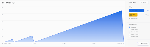
We can visualize the result with a quick chart in Snowsight showing on the x-axis the observation time in minutes and on the y axis how many minutes ago the last refresh happened. We can observe the freshness delay go up at a rate of 1 minute per minute and then crash down to 0 once a run completes.
Now that we have a freshness value for each minute, we can compare it to our objective and calculate the percentage of minutes that meets the objective.
We’ll wrap the previously final select in a CTE and add another step to calculate the percentage and get our final query. For our dashboard, we also add another query that counts the number of days with a percentage below 95%.
WITH completions AS (
    SELECT
        to_timestamp_tz('2024-03-01 01:00:00 +0000') AS interval_start,
        to_timestamp_tz('2024-03-01 01:05:00 +0000') AS interval_end,
        to_timestamp_tz('2024-03-01 01:10:00 +0000') AS completion
    UNION ALL
    SELECT
        to_timestamp_tz('2024-03-01 01:05:00 +0000') AS interval_start,
        to_timestamp_tz('2024-03-01 01:10:00 +0000') AS interval_end,
        to_timestamp_tz('2024-03-01 01:15:00 +0000') AS completion
    UNION ALL
    SELECT
        to_timestamp_tz('2024-03-01 01:10:00 +0000') AS interval_start,
        to_timestamp_tz('2024-03-01 01:15:00 +0000') AS interval_end,
        to_timestamp_tz('2024-03-01 01:25:00 +0000') AS completion
    UNION ALL
    SELECT
        to_timestamp_tz('2024-03-01 01:20:00 +0000') AS interval_start,
        to_timestamp_tz('2024-03-01 01:25:00 +0000') AS interval_end,
        to_timestamp_tz('2024-03-01 02:10:00 +0000') AS completion
),
minutes AS (
    SELECT
        convert_timezone(
            'UTC',
            DATEADD(
                MINUTE,
                SEQ4(),
                (SELECT MIN(completion) FROM completions)
            )
        ) AS timestamp
    FROM
        TABLE(GENERATOR(ROWCOUNT => 100))
    WHERE
        timestamp BETWEEN (SELECT MIN(completion) FROM completions)
        AND (SELECT MAX(completion) FROM completions)
),
freshness_per_minute AS (
    SELECT
        *,
        datediff(minute, completion, timestamp) AS processing_delay_minutes
    FROM
        minutes
    ASOF JOIN completions
    MATCH_CONDITION(
        minutes.timestamp >= completions.completion
    )
)
SELECT
    to_date(timestamp) AS completion_day,
    SUM(to_number(processing_delay_minutes < 15)) / COUNT(1) AS percentage_minutes_within_minutes_processing_delay_threshold
FROM
    freshness_per_minute
GROUP BY ALL;
| COMPLETION_DAY | percentage_minutes_within_minutes_processing_delay_threshold |
|---|---|
| 2024-03-01 | 50.8% |
Note that the percentage formatting was done for the article and running the query will return a decimal number. I never liked multiplying decimals by 100 to give percentages as I believe that’s a purely formatting detail, but feel free to do so in your version of the code.
Our example day didn’t go well, but rest assured that our pipelines are a lot more stable than this. I just thought the example would be boring without a good delay.
The big picture
We can now build visualizations to look at our SLO’s using the completion tables in a single Snowflake account. If we stopped here, we would be in a painful situation as we have Snowflake accounts in multiple regions. To have a centralized dashboard for our SLO’s, we use Snowflake replication to replicate this data to a centralized account. Following the ideas shown in the late runs example (adding the extra columns to the correct selects, partition by, and joins), we add dimensions for the account, region and pipeline name to present visualizations at different levels of granularity.
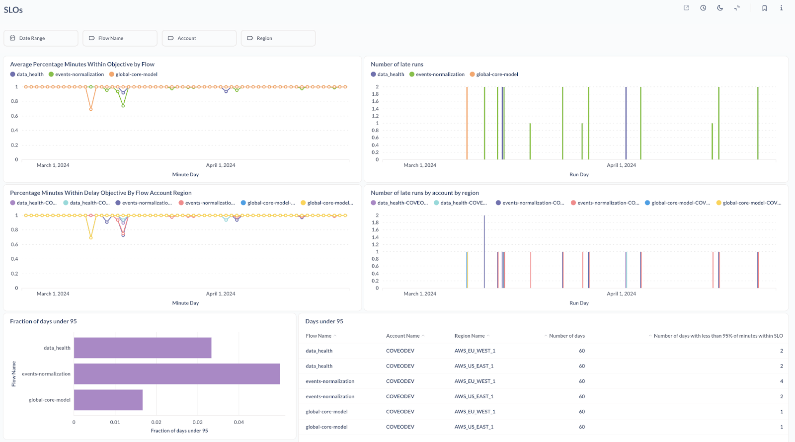
Using the queries explained in the article, we built the below dashboard in Metabase, dissecting our SLO performance from a few different angles. On the left we have the percentage of minutes within the freshness objective over time by day for our three main pipelines, and just below the same graph is broken down by Snowflake account. On the right, we have the number of late runs per day which can help us diagnose problems and focus our efforts on error recovery or avoidance (making sure runs don’t fail vs. starting new runs when they do). The bottom part shows a bigger picture counting the number of days when less than 95% of minutes are within the SLI.
Conclusion
In this article, we discussed the importance of providing SLO’s so that other teams can know what to expect from the data sources we provide, as well as helping us prioritize our efforts to make sure we meet these objectives. I then showed you how to leverage a table with interval completions and SQL functionality such as lag, generator, and asof join to measure our SLOs. In our case, we built the SLO dashboard at a time when we’re satisfied with the stability of our pipelines, but I encourage you to set it up first to motivate the effort and resources invested. We will definitely be doing it with our future pipelines.
If you’re passionate about software engineering, and you would like to work with other developers who are passionate about their work, make sure to check out our careers page and apply to join the team!